So you want to build an autoencoder? Great! This article will demonstrate how to build an autoencoder and use it to measure stock prices against an index. This technique is described in more technical terms here.

Once we’ve trained the autoencoder, we can use it to measure how well each component follows the other members of the index. This can be useful for finding deeper insights into an index, and doesn’t require a priori knowledge of the index price or the weighting of its components. Note, this is only one metric which one could use to determine how well one member of the group follows the group overall. Another might be Pearson Correlation.

Github repository

To follow along with the code in this tutorial, please download the corresponding repository on Github:

git clone git@github.com:lukesalamone/stock-data-autoencoder.git
cd stock-data-autoencoder
pip install -r requirements.txt

What is an autoencoder?

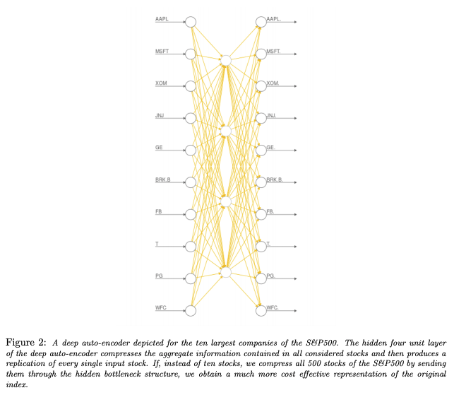
An autoencoder is a neural network which encodes information back to itself. The structure of the network is such that the input layers (the “encoder”) will be large compared to the hidden layers (the “code”), forcing the network to compress information inside its hidden layers.

The idea of our autoencoder is that we would like to encode stock price information back to itself while discarding trends that aren’t important. To do this, we will feed our network stock price data and ask the network to return those prices to us as outputs. Component stocks which are important to the index will be preserved well and thus be highly accurate, while components which are less important will not be well-preserved. We will measure the performance of the network on each component using mean squared error.

The model

We will use an autoencoder with a number of inputs and outputs equal to the number of component stocks in our index. For this exercise, we will use the S&P 500 index which contains 505 components. This means our input and output size will be 505. We will also use a hidden layer with 5 units.

class StonksNet(nn.Module):
  def __init__(self, size):
    super().__init__()
      self.fc1 = nn.Linear(in_features=size, out_features=5)
      self.out = nn.Linear(in_features=5, out_features=size)

  def forward(self, x: Tensor) -> Tensor:
    x = F.relu(self.fc1(x))
    x = F.relu(self.out(x))
    return x

The data

We will use daily stock prices downloaded using yfinance. This data is readily available online and I recommend downloading it for yourself. We will use data between January 1, 1991 to January 1, 2021 (30 years of data).

To download the S&P 500 stock data please run gather_stocks.py from the project directory:

python gather_stocks.py

This will download all 505 components into the stock_data directory. Data will also be cleaned such that each component has the same number of days, which will be important when feeding it into the model.

Training the model

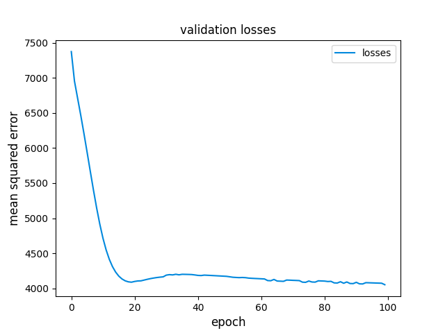
The model itself is a simple feed-forward neural network. As such, we use a standard training loop to train the model. We don’t expect the loss to ever fall to zero during training since it is impossible for the network to perfectly encode and decode so many inputs into so few hidden code units. Some information will inevitably be lost. In my training, validation losses bottomed out at around 4000, but yours may be different depending on the initialization of your autoencoder.

Ranking components

Finally we’re ready to rank the components of the S&P 500 for “closeness”. After running python train_model.py you will see the best and worst components as scored by the autoencoder. Here were my results, yours may be different.

best 5 results:
DRE: 16.66
LNT: 37.27
MU: 38.88
HOLX: 43.18
CERN: 47.46

worst 5 results:
HUM: 105244.19
SHW: 108542.73
LMT: 113654.48
C: 357073.88
NVR: 10955169.00

Future research

Upon inspection, it appears that better results might be achieved if we normalize the stock data before training. It appears that stocks with higher prices and higher volatility tended to perform worse than those with tight price ranges. In a way this is expected, since the autoencoder will naturally have a harder time modeling large values with a limited set of hidden units. However, normalizing the prices into similar ranges might be an interesting exercise to see if we can squeeze even more out of the model.