7 minutes
Summary: Deep & Cross Net v2
Paper link: https://arxiv.org/pdf/2008.13535
Learning to rank is an important problem in many machine-learning products such as search, recommendation, and advertising. Originally, many machine learning systems used simple logistic regression models, but it quickly became apparent that combining two or more features together was even better. This is called feature crossing.
A lot of research and engineering work has gone into learning useful feature crosses. The fundamental problem is that although higher-order feature crosses can be more informative, they are also more sparse, and the number of high order features grows exponentially. Some attempts to address this have been:
| Architecture | Description |
|---|---|
| Wide & Deep network | Contains a wide linear model to capture feature interactions and a deep neural net (DNN) to capture nonlinear relationships. |
| DeepFM | Combines a FM component to capture second-order feature interactions and a DNN to capture higher-order interactions. |
| xDeepFM | Extends DeepFM by adding a compressed interaction network to model high-order vector-wise feature interactions. |
| DLRM | Uses a DNN for dense features, an embedding lookup for sparse features, dot product interaction layers, and a final DNN. |
| PNN | Uses a product layer to explicitly model pairwise feature interactions, followed by a neural net. |
| AutoInt | Uses multi-head self-attention to model feature interactions, followed by a DNN. |
| DCN | Explicitly applies feature crosses with a Cross network, followed by a DNN. |
DCNv2
DCNv2 improves on the original DCN architecture in a few important ways. First, it uses a more expressive feature cross formula. Second, it introduces matrix factorization to dramatically reduce the required number of parameters in the model. Finally, the authors also introduce a gated mixture of experts setup to take advantage of the parameter savings.
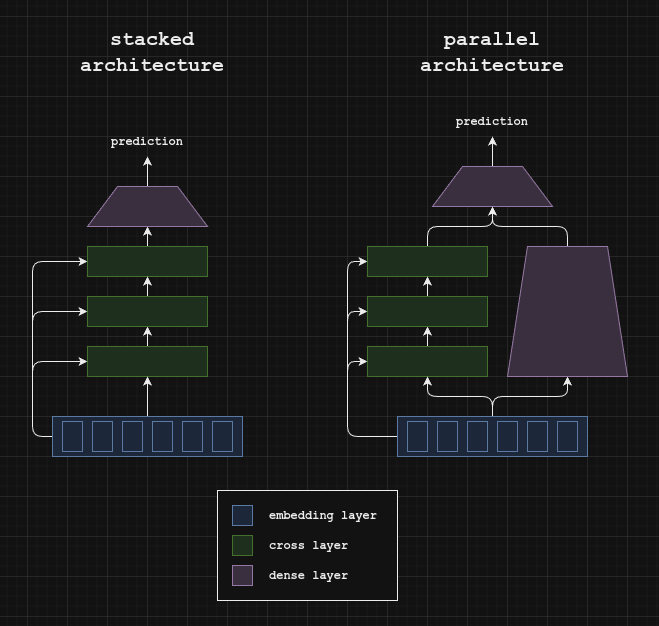
DCNv2 can be implemented with a stacked (i.e. serial) architecture or a parallel architecture.
Embedding layer
To create the embedding layer, all features are concatenated together to create a tensor with shape batch size x embedding size. For one-hot encoded categorical features, they can be projected to a much lower dimensionality with a learned matrix (i.e. a single dense layer with no bias term).
One convenient property of this embedding scheme is that feature order doesn’t matter. All features will be crossed with all other features, so we don’t need to worry about the way that features are added and removed.
Cross Net
The formula for a single cross operation is
"""
Dimension key:
    B: batch size
    D: embedding dimension

Params:
    x_0: original embedding, shape BD
    x_i: i-th embedding, shape BD
    weight_i: i-th learned weight matrix, shape DD
    bias_i: i-th learned bias term, shape D

Returns:
    The residual embedding after i+1 cross operations
"""

def cross(x_0, x_i, weight_i, bias_i):
    x_0 = x_0.unsqueeze(-1)         # (B, D, 1)
    x_i = x_i.unsqueeze(-1)         # (B, D, 1)
    bias_i = bias_i.unsqueeze(-1)   # (D, 1)

    kernel = weight_i @ x_i     # (D, D) @ (B, D, 1) = (B, D, 1)
    kernel = kernel + bias_i    # (B, D, 1) + (D, 1) = (B, D, 1)

    result = x_0 * kernel + x_i # (B, D, 1)
    return result.squeeze(-1)   # (B, D)
Note that the weight_i @ x_i + bias_i term is equivalent to a fully-connected neural network layer with no activation. To this result, we element-wise multiply the original embedding, then add the i-th embedding.
Low rank approximation
Of course, with high embedding dimensionality, the weight matrix can easily grow to millions of parameters, and we need a weight matrix for each of the cross operations. A common technique to reduce the number of parameters is to use a low rank approximation of the weight matrix. In other words, we can replace the weight @ x operation with weight_u @ (weight_v @ x)
In particular, rather than requiring DxD parameters for each cross operation, we will now only need DxR + RxD = 2xRxD parameters, where R is the low-rank approximation dimension. So if R is less than half of D, we can save parameters using this technique.
"""
Dimension key:
    B: batch size
    D: embedding dimension
    R: low rank dimension

Params:
    x0: original embedding, shape BD
    xi: i-th embedding, shape BD
    weight_u_i: i-th learned weight matrix, shape DR
    weight_v_i: i-th learned weight matrix, shape RD
    bias_i: i-th learned bias term, shape D

Returns:
    The residual embedding after i+1 cross operations
"""

def low_rank_cross(x_0, x_i, weight_u_i, weight_v_i, bias_i):
    x_0 = x_0.unsqueeze(-1)         # (B, D, 1)
    x_i = x_i.unsqueeze(-1)         # (B, D, 1)
    bias_i = bias_i.unsqueeze(-1)   # (D, 1)

    kernel = weight_v_i @ x_i       # (R, D) @ (B, D, 1) = (B, R, 1)
    kernel = weight_u_i @ kernel    # (D, R) @ (B, R, D) = (B, D, 1)
    kernel = kernel + bias_i        # (B, D, 1) + (D, 1) = (B, D, 1)

    result = x_0 * kernel + x_i     # (B, D, 1)
    return result.squeeze(-1)       # (B, D)
Mixture of low-rank experts
The parameter savings from using low-rank approximations of the weight matrices can be reinvested into additional parameters. In particular, if we have a gating function G(x) we can use it to decide between a group of “experts” which are themselves low-rank Cross networks.
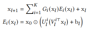
A mixture of experts consists of a gating function and an expert function. The gating function determines the weight of the expert function.
Note that setting G(x)=1 and K=1 reduces the mixture of experts to the original low-rank DCN architecture.
Analysis of hyperparameters
The number of cross layers (i.e. cross depth), the choice of low-rank approximation, and the number of experts can each have a large effect on the model performance. For the depth of the crosses, the researchers found that performance improved with the number of cross layers, but diminishing returns as depth increased.
The behavior of the matrix rank was interesting. For very low rank, the model performed similarly with other baselines. However, increasing from rank 4 to 64 showed dramatic performance improvement, and notable but lesser improvement afterwards. This suggests there is some “elbow” (the authors call this a threshold rank) which maintains good performance without consuming too many parameters.
For the number of experts, the researchers found that the total rank sum of all of the experts was the main contributing factor for performance. In other words, 1x256, 4x64, 8x32, 16x16 and 32x8 all performed similarly. They hypothesized that their simple gating function was responsible for this.
Results on synthetic datasets
To better understand how the DCN, DCNv2 and DNN are able to model cross interactions, the authors created synthetic functions for the various architectures to learn. They created three classes of functions with increasing difficulty to learn.
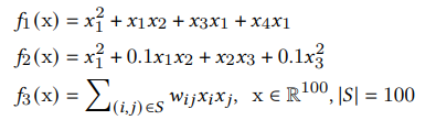
Synthetic functions of increasing difficulty to be learned by DCN, DCNv2 and DNN.
Note that the third equation can be modeled by a single cross operation.
In their experiments, the authors found:
- The DCN consistently used the fewest parameters (maximum of 300 parameters) and was able to accurately model the simpler functions, but was unable to accurately model the third, most complicated function with a single layer. However, since a single layer was only 300 parameters, experimenting with a larger model would have been interesting.
- The DNN used the most parameters (up to 758k parameters) and was unable to model any of the functions as accurately as either DCN or DCNv2.
- The DCNv2 used up to 10k parameters for the most complex function and achieved the lowest RMSE loss by far.
The authors also directly compared DCNv2 models with varying numbers of layers with a traditional DNN in modeling a more complex function containing sine terms and polynomials of order 1-4 and found that DNNs are highly inefficient in modeling higher order interactions.
Results on Criteo
Criteo is a popular click-through-rate (CTR) prediction dataset containing 7 days of user logs. It contains 13 continuous features and 26 categorical features.
On Criteo, DCN-v2 (best setting using two layers) had a 0.21% better AUC than a DNN baseline. DCN-Mix (best setting using 3 layers, 4 experts, and low rank of 258) was 0.17% better on AUC than the DNN baseline.
Results on MovieLens-1M
MovieLens-1M is a popular dataset for recommendation systems research, containing one million samples of [user-features, movie-features, rating] triplets. The task was treated as a regression problem. Ratings of 1 and 2 were set to 0 and 4 and 5 were set to 1. 3s were removed.
On MovieLens, DCN-V2 was 0.24% better on AUC than the DNN baseline. DCN-Mix was even better, at +0.39% over the DNN baseline.