4 minutes
How does HNSW work?
Suppose we have a vector database with a billion items in it (the haystack). And suppose we are looking for K vectors, the needles which maximize some similarity function. (In the case of cosine similarity or euclidean distance, we may be maximizing 1-distance(x,y).) And also suppose that we’d like to do this quickly.
Naive and semi-naive approaches
One approach might be to compare every vector and take the argmax. In that case, for vectors of length D our runtime will be 1 billion x D.
def search(needle, haystack, arg_k=1):
    # normalize needle and haystack vectors
    needle /= np.linalg.norm(needle)
    haystack /= np.linalg.norm(haystack, axis=1, keepdims=True)

    # compute cosine similarities
    similarities = np.dot(haystack, needle)

    # get the indexes of the top k elements
    idx_topk = np.argpartition(a, -k)[-k:]

    # return haystack vector with highest cosine similarity
    return haystack[idx_topk]
In practice, there are some optimizations we can try which can increase the practical speed of this operation:
- We can parallelize computations on-device with SIMD or BLAS.
- We can parallelize computations on-device with GPU.
- We can parallelize across cores for machines with multiple cores.
- We can parallelize across devices. For example, partitioning the database across 10 clusters, finding a “winner” from each cluster, and then repeating the search across the 10 winners.
There are also some relatively simple but “destructive” techniques we can also try:
- We can try pruning the dataset in some way beforehand. For example, maybe we don’t need to consider old or unpopular vectors.
- We can try reducing the dimensionality of the vectors with something like PCA.
- We can try quantizing the vectors e.g.
f64->f16reduces memory requirements 4x. (Usually this requires quantization-aware training.)
Hierarchical Navigable Small Worlds (HNSW)
Sometimes linear time is still too slow. In that case, we can consider an approximate solution, where some acceptable percent of vectors returned are actually not in the top K nearest neighbors. This is called approximate nearest neighbors (ANN). If we have a large system, it’s possible to use another more precise model to rerank the vectors results anyways. In that case, we just need to set K large enough to reliably include the vectors we really need.
ANN algorithms typically come in three flavors: graph based approaches, space partitioning based approaches, and hash based approaches. If your dataset is large enough, you might add compression (e.g. product quantization) on top of it.
Intuition
HNSW is a bit of a Six Degrees of Kevin Bacon approach. I’ll give what I think this is a fairly good intuition for how it works.
Suppose you have 1,000 friends and you’d like to know which five of them live closest to a landmark like the Golden Gate Bridge. You don’t have everyone’s exact address, but each friend keeps a list of their close friends’ addresses. You might start with a friend who lives in the US. From there, you check their friends to find who lives closest to the target, and then search among their friends for someone even closer. By using a hierarchical approach, you don’t need to search through everyone, just those likely to be closest.
In the analogy, the Golden Gate Bridge is the “needle” and the friends are the “haystack”. This is a pretty efficient method, but of course it is possible to miss a node if their friend wasn’t linked to an earlier friend.
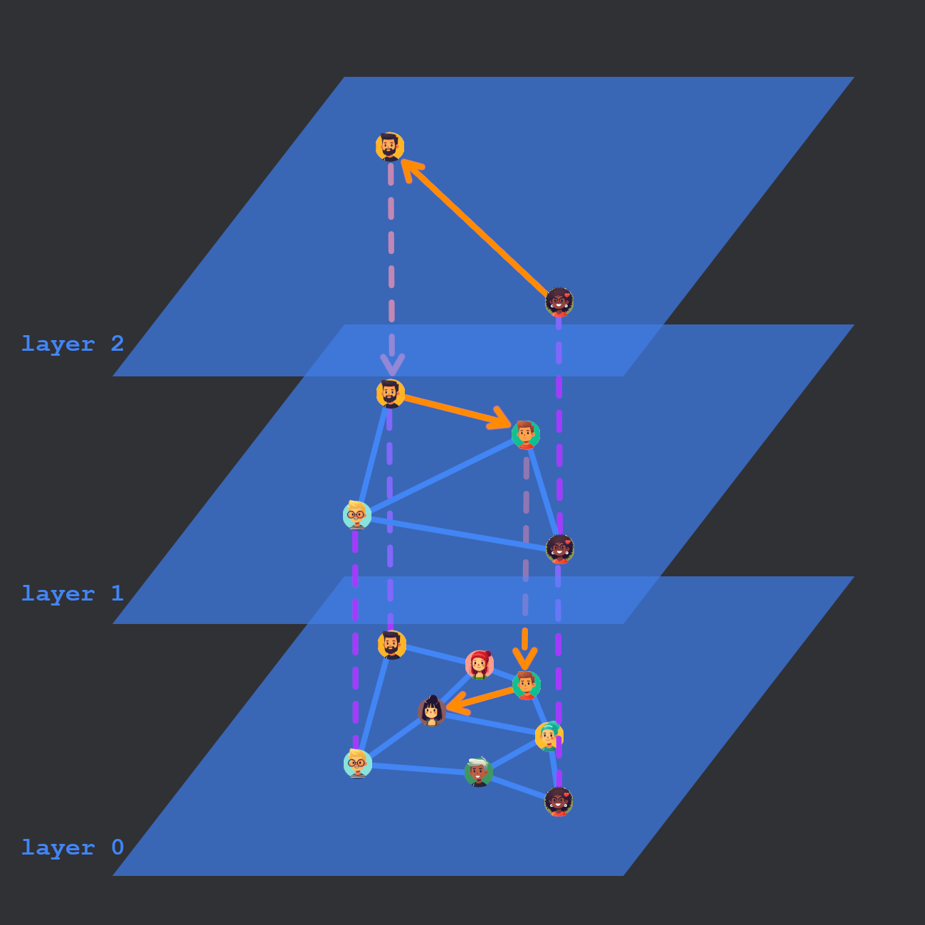
HNSW uses a multi-layered graph for efficient nearest neighbor search.
Searching
Searching is fairly straightforward. Start from an entry point (maybe a random point) in the top layer. For each of the neighbors of the entry point, compute the distance between the query and that point. If any of the neighbors are closer to the query, hop to that neighbor and repeat the process. Select the closest point and go to the next layer down. We keep searching until we reach layer 0.
To compute the K nearest neighbors during search (with K > 1) we simply maintain a min heap, and add all nodes considered during the search. The number of nodes returned in this search (K) is also known as ef_search in the HNSW paper.
Addition
To add a vector X, we start by computing the highest layer L the node will appear in. L is randomly selected using an exponentially decaying probability. (All nodes appear in level 0, but can have skip links to higher levels.) Next, starting from the top layer, we traverse the graph structure as if we were searching for X.
Once we reach layer L from earlier, we begin to make connections. Connections can be made with previously found nearest neighbors or nearest neighbors on the current layer. The number of nearest neighbors to consider connections with is controlled by the ef_construction parameter. The number of links to actually create is controlled by the parameter M.
Performance considerations
- HNSW can require a large amount of memory. This can be reduced with product quantization, a lossy vector compression method.
- Adding new elements is slow. There is a tradeoff between index quality and time required to build the index controlled by
ef_construction.
More information about HNSW parameters can be found here.