6 minutes
Learning the Haystack
Embeddings, or vector representations of a document (which could be a piece of text, image, sound, etc.), can be extremely useful for making sense of large datasets. They transform information into a vector space such that their distance corresponds to their similarity.
Enterprising readers might be asking themselves how to get these vectors (also known as embeddings) in the first place. One way is to simply pay for them. This isn’t ideal for a couple of reasons:
- It can be expensive. You’ll need to pay once to embed each document, and separately for each query. If you have a large corpus, it can be cost-prohibitive. At the time of writing, OpenAI charges about $130 per million tokens (around 1000 paragraphs) for their largest model.
- “Similarity” may mean different things depending on your use case. For example, suppose we are retrieving documents for customer support. For the embedding model to learn that two documents share user behavior characteristics (i.e. two documents were opened by support agents in the same session), that information needs to be available in the training process.
Below is an overview of three of the main training regimes I have used for creating embeddings. For more information and in-depth examples, I highly recommend the loss overview page of the Sentence Transformers library. Generally speaking, there are three categories of methods: unsupervised methods, contrastive learning methods (positive/negative labels), and regression methods (floating-point labels).
Autoencoders
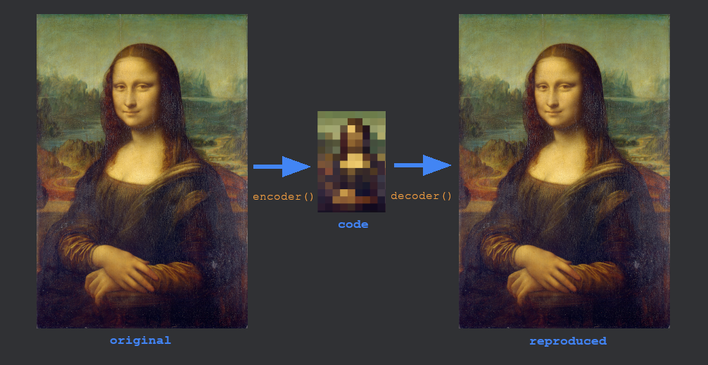
An autoencoder uses a bottleneck to reduce the dimensionality of the input.
One approach for vectorizing a document, image, or other blob of information is to simply use an autoencoder. An autoencoder is a function which learns a lossy compression function. It can be considered an unsupervised method since each item is its own label.
However, although they are conceptually pretty simple, autoencoders aren’t always best. They may learn an efficient representation of your document, but it may be wasting a lot of space on things you don’t care about.
For example, if it was reproducing a picture which contained a TV showing static, you may not care exactly what the static looks like, just that it has static. So it’s probably a waste of space to try to reproduce every pixel of static. Likewise, if it were encoding people, it might be really important to you that the people have 5 fingers. Unfortunately, the autoencoder wasted too much space encoding the TV and not on boring details like numbers of fingers.
See also: the “noisy TV problem”
Fine-tuning with Sentence Transformers
The applicability of the next few methods will depend on the format of your data and labels.
Here is a simple example for creating text embeddings with sentence-transformers using ContrastiveLoss:
from sentence_transformers import (
  SentenceTransformer,
  SentenceTransformerTrainer
)
from sentence_transformers.losses import ContrastiveLoss
from datasets import Dataset

model = SentenceTransformer('all-MiniLM-L6-v2')
train_dataset = Dataset.from_dict({
    "sentence1": [
      "I feel the need...",
      "Life is like a box of chocolates."
    ],
    "sentence2": [
      "...the need for speed!", # similar
      "Here's Johnny!" # dissimilar
    ],
    "label": [1, 0],
})

trainer = SentenceTransformerTrainer(
    model=model,
    train_dataset=train_dataset,
    loss=ContrastiveLoss(model),
)
trainer.train()
And to generate the embedding:
embedding = model.encode(["There's no crying in baseball!"])
print(embedding.shape) # (1, 384)
Contrastive Learning: Triplet loss
Triplet loss explicitly learns embeddings to be used in cosine similarity or euclidean distance (L2 norm) comparison. It uses triplets of the form (A, P, N), where A is an anchor, P is a positive example which is similar to A, and N is a negative example which is dissimilar to A. For example if we wanted to learn embeddings for songs, we might say a positive example is a spectrogram clip from the same artist as the anchor, and a negative sample is from a different artist.
$$ \text{L} = \sum_{i=1}^N \text{max} \left(0, cos( f(a_i) - f(p_i) ) - cos( f(a_i) - f( n_i )) + m \right) $$
for cosine similarity or for euclidean distiance,
$$ \text{L} = \sum_{i=1}^N \text{max} \left(0, \lVert f(a_i) - f(p_i) \rVert_2 - \lVert f(a_i) - f( n_i ) \rVert_2 + m \right) $$
In other words, we enforce that the distance between the anchor and the negative sample is greater than the distance between the anchor and the positive sample plus some margin. For cosine similarity, what this would look like is that your vectors appear as points on the perimeter of a high-dimensional clock face (i.e. the surface of an N-dimensional hypersphere). Positive samples grow closer to the anchor while the negative samples are pushed away. The higher the margin, the closer positive samples will be pushed together.
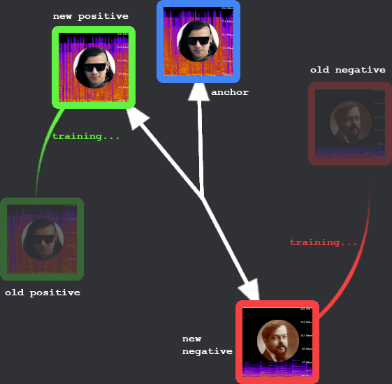
Learning to differentiate Bangarang and Clair de lune. Triplet loss pushes positive examples closer to the anchor and negatives farther away. Some say Claude DeBussy was the Skrillex of 1890.
Contrastive learning: Contrastive loss
If you have binary labels, you can use contrastive loss. It works with positive pairs (anchor, positive) and negative pairs (anchor, negative), denoted with a binary label. In the original paper, $ y \in [1,0] $ is the label indicating the desired distance between the points (not whether they are similar).
Like triplet loss, contrastive loss also includes a margin parameter. For dissimilar pairs, a loss is incurred only if their predicted distance falls within the margin’s radius.
$$ \text{loss} = \frac{(1-y_{i})(D_{W_i})^2 + y_i \left( \text{max}(0, m - D_{W_i}) \right) ^ 2 }{2} $$
Where $ D_{W_i} $ is euclidean distance between the two embeddings of sentences $ a_i $ and $ b_i $:
$$ D_{W_i} = \lVert f(a_i) - f(b_i) \rVert _{2} $$
Note that triplet loss is often confused with contrastive loss, but they are not the same.
Regression: Cosine similarity loss
If you already have some numerical labels for the similarity of two pieces of text, you can compute mean squared error between their predicted cosine similarity and the actual similarity.
For pairs of sentences ai and bi and label yi,
$$ \text{loss} = \frac{1}{N} \sum_{i=1}^{N} \left[ cos\left(f(a_{i}), f(b_{i})\right) - y_{i} \right] ^ 2 $$
Regression: CoSENT loss
CoSENT loss is an improved version of cosine similarity learning which makes better use of in-batch values. For a batch with size N it makes up to Nx(N-1)/2 predictions. (I.e. for a batch size of 10 we make up to 45 predictions rather than the 10 in Cosine Similarity Loss.) It is essentially a ranking loss, taking advantage of the knowledge of the relative similarities within the batch.
$$ \text{loss} = \log \left( 1 + \sum_{\text{sim}(i,j) > \text{sim}(k,l)} e^{\lambda (\cos(k, l) - \cos(i, j))} \right) $$
Experiments have shown improved performance over Cosine Similarity loss.